Elm-stat

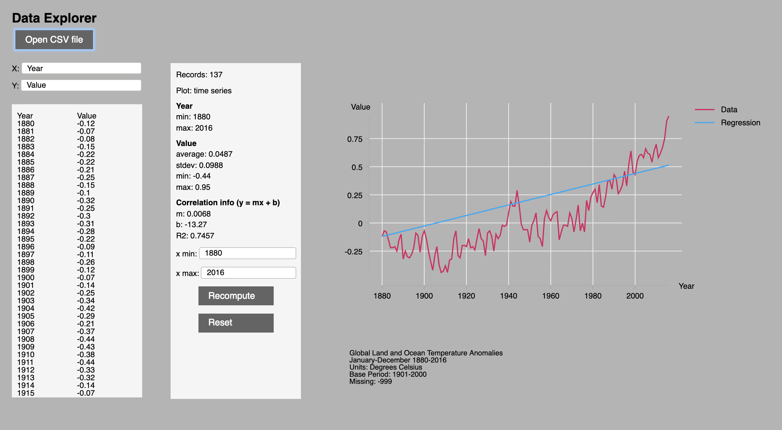
This package is for doing statistics and graphs for 2-column csv files.
The image above displays an analysis of time series data. It is computed by the app in the examples folder using this elm-stat library. See the Demo App to try the app out on line.

The API

There are two modules, Stat, for computing statistics of 2-D data, and CsvData, for extracting Csv data from a text string and for extracting 2-D data from Csv. The Stat module has functions for computing statistical measures such as the mean and standard deviation of the x or y values, coefficients for the linear regression line, etc.

Let's import both modules to see how they work.

> import Stat exposing(..)
> import CsvData exposing(..)

Here is an extract of the data in data/temperature-anomalies.csv:

> rawdata = "year,value\n1880,-0.12\n1881,-0.07\n1882,-0.08\n1883,-0.15\n"
"year,value\n1880,-0.12\n1881,-0.07\n1882,-0.08\n1883,-0.15\n"
    : String

Next, transform it to csv using CsvData.get. This function is \str -> Just <| Csv.parse <| filter str, where Csv is from zgohr/elm-csv. The function CsvData.intelligentGet does additional checking and manipulation, e.g., it tries to return the text header that many data files have.

> maybeCsv = CsvData.get rawdata
    Just { headers = ["year","value"], records = [["1880","-0.12"]
          ,["1881","-0.07"],["1882","-0.08"],["1883","-0.15"]] }
    : Maybe Csv.Csv

For this example, we extract the value by hand:

> csv = { headers = ["year","value"], records = [["1880","-0.12"],
         ["1881","-0.07"],["1882","-0.08"],["1883","-0.15"]] }
    : { headers : List String, records : List (List String) }

With the csv data in hand, we convert it to a list of points:

> data  = CsvData.getPointList 0 1 csv
    [{ x = 1880, y = -0.12 },{ x = 1881, y = -0.07 },{ x = 1882, y = -0.08 }
    ,{ x = 1883, y = -0.15 }]
    : Data

From a Data = List Point value, one can compute statistics:

> Stat.average .y data
  Just -0.105 : Maybe Float
> Stat.stdev .y data
  Just 0.0013666 : Maybe Float

The statistics function computes a package of statistical measures, including left and right endpoints for the regression line for the data. These can be used to superimpose the regression line on the plot of the data. This is done in the demo app using terezka/line-charts.

> Stat.statistics data
  Just { b = 18.7099, leftDataPoint = { x = 1880, y = -0.12 }
  , leftRegressionPoint = { x = 1880, y = -0.09 }
  , m = -0.009999, n = 4, r2 = 0.12195
  , rightDataPoint = { x = 1883, y = -0.15 }
  , rightRegressionPoint = { x = 1883, y = -0.1200 }
  , xMax = 1883, xMean = 1881.5, xMin = 1880, xStdev = 1.29099
  , yMean = -0.105, yStdev = 0.036968 }

The Demo app

Code for the demo app is in ./examples. There is an online version at Data explorer

The data used in the example in the file data/temperature-anomalies.csv in this repo. It is a list of global temperature anomalies for the period 1880-2017 from www.climate.gov. The annual temperature anomaly is the difference between the global mean temperature and the long-term mean global temperature. For this data set, the long-term mean is computed for the period 1901-2000. Here is what the data looks like:

Global Land and Ocean Temperature Anomalies, January-December
Units: Degrees Celsius
Base Period: 1901-2000
Year,Value
1880,-0.12
1881,-0.07
...
2015,0.91
2016,0.95